Explore treatment of intra-episode siblings • Pv3Rs

As the following example illustrates, Pv3Rs sums over graphs with cliques of three or more intra-episode siblings when MOIs used by the Pv3Rs model exceed two. However, when the data input via the y argument of compute_posterior() are as diverse as the MOIs used by the Pv3Rs model, graphs with cliques of three or more intra-episode sibling parasites have zero likelihood; when MOIs used by the Pv3Rs model are more diverse than the data input via the y argument of compute_posterior() (e.g., because the user inputs elevated MOIs into compute_posterior()), graphs with cliques of three or more intra-episode siblings have non-zero likelihoods. In either case, provided MOIs used by the Pv3Rs model are based on estimates from per-episode parasite genetic data generated and analysed in bulk (i.e., not single-cell data), groups of three or more not-half intra-episode siblings collapse to groups of two because

MOI estimates based on maximum per-marker allele counts are at most two for groups of three or more not-half siblings because groups of not-half siblings can draw from at most two parental alleles per marker.
MOI estimates based on heteroallelic marker counts count at most two for groups of three or more not-half siblings because data from a group of not-half siblings can be at most as diverse across markers as the two parental genotypes from which they draw.

Example of a group of four intra-episode siblings collapsing to two

Before showing how groups of intra-episode siblings collapse to pairs of intra-episode siblings, we write a function to simulate data of a given allelic richness (marker cardinality) on an enrolment episode comprising a stranger plus a group of four siblings, two from one oocyst, two from another, all drawing from the same two unrelated parental genotypes, and a recurrence with one sibling. Technically, the enrolment episode contains five genetically distinct genotypes and thus has a MOI of five.

simulate_data <- function(marker_cardinality){
  
  # Magic numbers / quantities
  set.seed(5) # For reproducibility
  n_markers <- 200 # Number of markers
  n_strangers <- 3 # Number of stranger parasites
  n_oocysts <- 2 # Number of oocysts to draw from
  
  # Derived quantities
  alleles <- letters[1:marker_cardinality]
  markers <- paste0("m", 1:n_markers) # Marker names
  
  # Uniform allele frequencies 
  fs <- sapply(markers, simplify = FALSE, 
               function(m) setNames(rep(1/marker_cardinality, marker_cardinality), alleles))
  
  # Sample strangers
  strangers <- sapply(1:n_strangers, function(i) {
    sapply(markers, function(t) sample(names(fs[[t]]), size = 1, prob = fs[[t]]))
  })
  
  # Designate strangers
  parents <- strangers[, 1:2]
  
  # Map the markers to chromosomes. Assume equally sized chromosomes — reasonable
  # if and only if we later assume an equal number of crossovers per chromosome
  chrs_per_marker <- round(seq(0.51, 14.5, length.out = n_markers))
  
  # Sample parental allocations dependently per-oocyst 
  cs <- lapply(1:n_oocysts, function(o) recombine_parent_ids(chrs_per_marker))
  
  # Construct children from parental allocations 
  all_children <- lapply(1:n_oocysts, function(o) {
    oocyst_chidren <- sapply(1:n_markers, function(i) {
      sapply(1:ncol(cs[[o]]), function(j) parents[i,cs[[o]][i,j]])
    })
    colnames(oocyst_chidren) <- markers
    return(oocyst_chidren)
  })
  
  # Make enrolment infection
  enrol <- apply(rbind(all_children[[1]][1:2,], 
                       all_children[[2]][1:2,], 
                       strangers[,3]), 2, unique, simplify = F)
  
  # Make paired data
  data <- list(enrol = enrol, recur = as.list(all_children[[1]][1,]))
  
  return(list(data = data, fs = fs))
}

However, MOI estimates based on maximum per-marker allele counts are three and one when markers are polyallelic:

polyallelic <- simulate_data(10) 
determine_MOIs(polyallelic$data)
#> [1] 3 1

And two and one when markers are biallelic:

biallelic <- simulate_data(2) 
determine_MOIs(biallelic$data)
#> [1] 2 1

Suppose we estimate MOIs of 3 and 1 for the biallelic data using an external software that exploits heteroallelic marker counts (rather than the maximum number of per-marker alleles), and input those external estimates into compute_posterior. Providing data are simulated on a large number of markers (200 above), we recover almost exactly the same posterior probabilities using both the

polyallelic data without user-specified MOIs
biallelic data with user-specified MOIs three and one

ppost <- suppressMessages(compute_posterior(y = polyallelic$data, 
                                            fs = polyallelic$fs, 
                                            return.logp = T))
bpost <- suppressMessages(compute_posterior(y = biallelic$data, 
                                            fs = biallelic$fs, 
                                            MOIs = c(3,1), return.logp = T))

ppost$marg
#>               C         L             I
#> recur 0.6666667 0.3333333 2.708985e-116
bpost$marg
#>               C         L            I
#> recur 0.6666663 0.3333337 4.625927e-18

However, given the polyallelic data the likelihoods of the following graphs with cliques of three intra-episode siblings are zero:

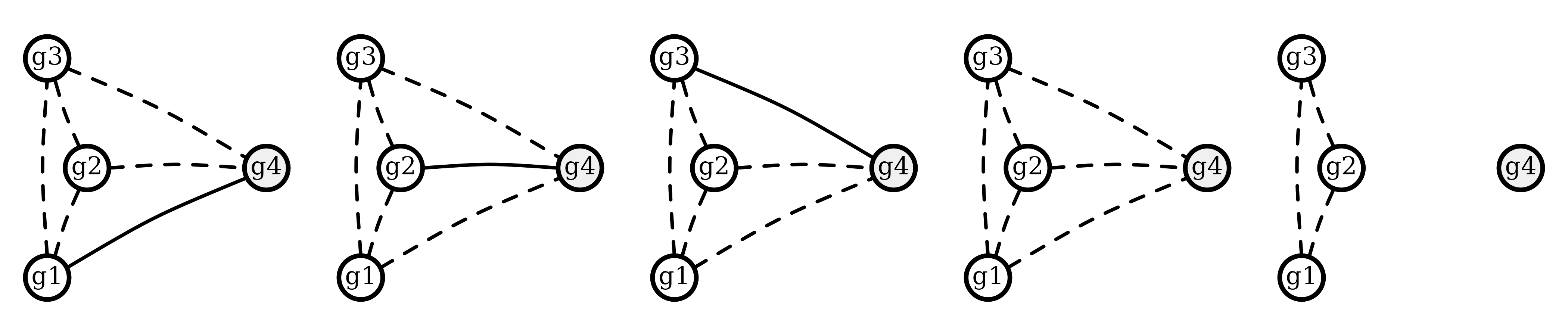
Whereas, all relationships have non-zero likelihoods given the biallelic data:

llikes <- sapply(bpost$RGs, function(RG) RG$logp) # Extract log likelihoods
any(is.infinite(llikes)) # Are there any minus infinity log likelihoods?
#> [1] FALSE

Contribution to upper bounds

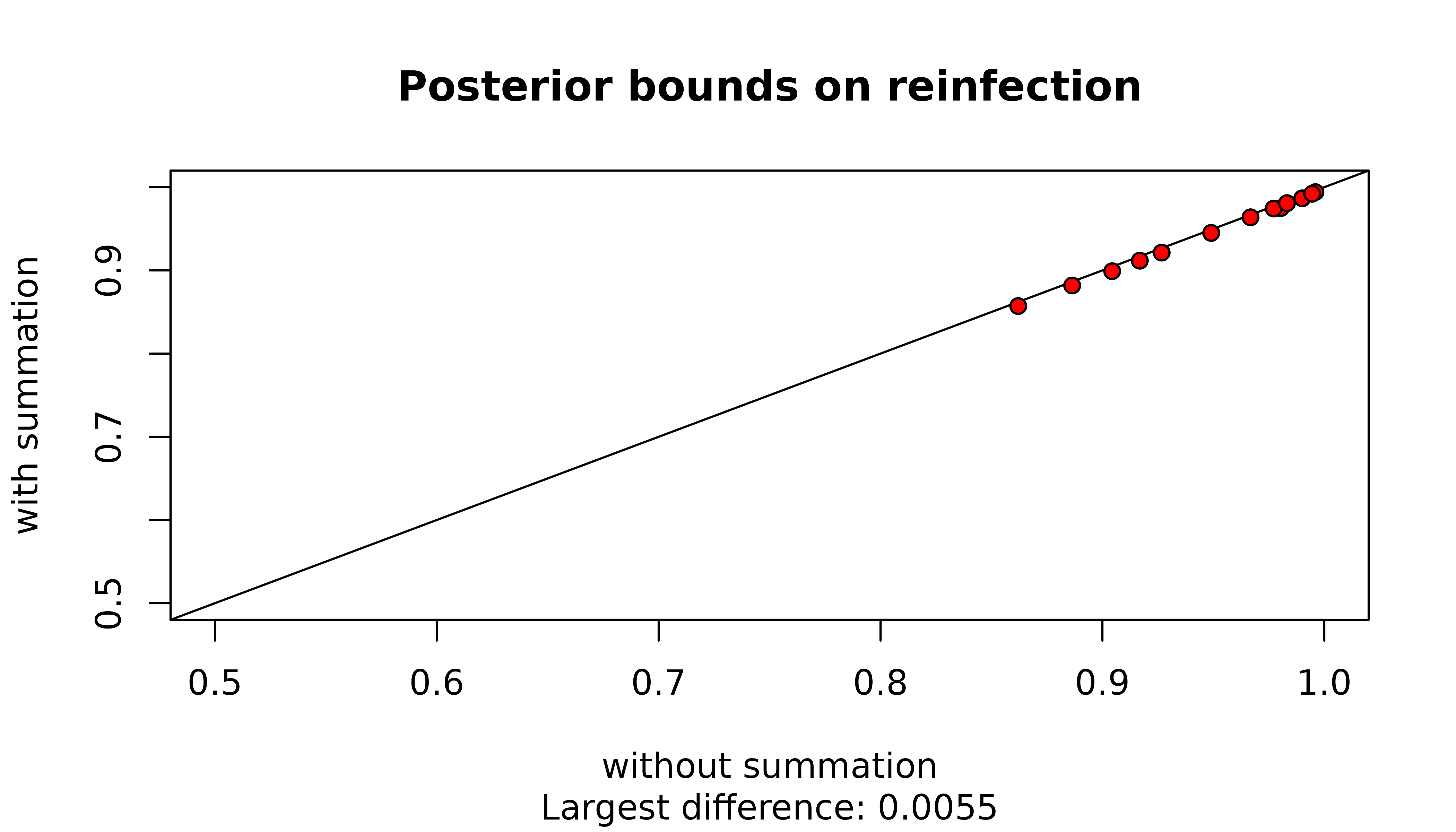
The summation over graphs with cliques or three or more siblings is possibly redundant given these graphs have no practical support. Even when these graphs have zero likelihood, they contribute to maximum probabilities of recrudescence / reinfection through the conditionally uniform prior on graphs. However, for upper bounds on the probability of reinfection / recrudescence given a single recurrence the contribution is very small, especially for reinfection:

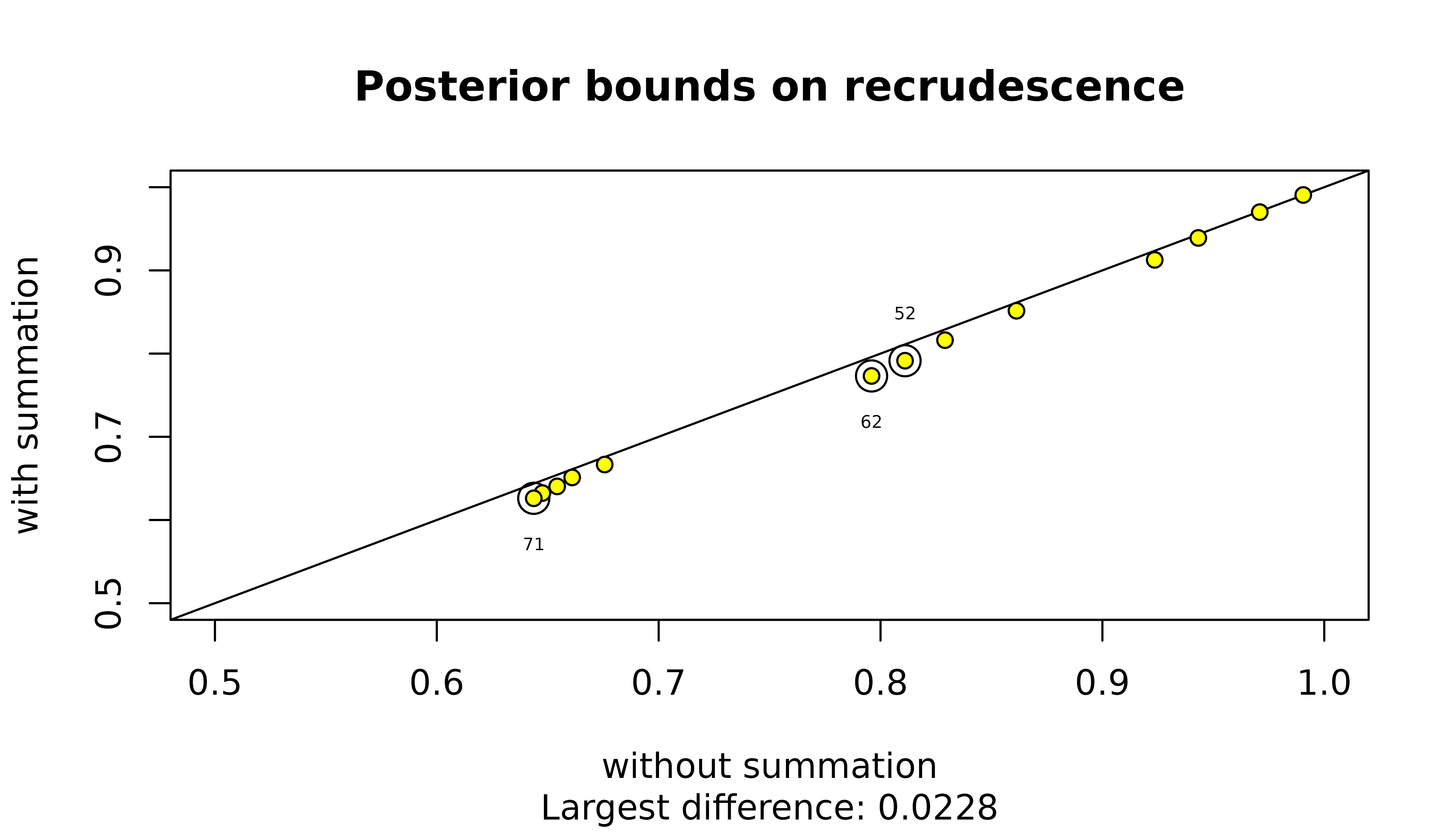
For recrudescence, 3 MOI vectors (circled below) result in an absolute difference greater than 0.0175. They are those that feature large MOIs (MOI vectors 52, 62, 71) and thus those whose graph spaces include graphs with the largest cliques of intra-episode siblings.

The contribution is likely smaller for all vectors of three or more MOIs that are computationally feasible under Pv3Rs because their constituent MOIs are necessarily less than 7 (computationally feasible MOI vectors are those where the total genotype count is at most eight).