Compute posterior probabilities of P. vivax recurrence states

Computes per-person posterior probabilities of P. vivax recurrence states — recrudescence, relapse, reinfection — using per-person genetic data on two or more episodes. For usage, see Examples below and Demonstrate Pv3Rs usage . For a more complete understanding of compute_posterior output, see Understand posterior probabilities.

Note: The progress bar may increment non-uniformly (see Details); it may appear stuck when computations are ongoing.

Usage

compute_posterior(
  y,
  fs,
  prior = NULL,
  MOIs = NULL,
  return.RG = FALSE,
  return.logp = FALSE,
  progress.bar = TRUE
)

Arguments

y: List of lists encoding allelic data. The outer list contains episodes in chronological order. The inner list contains named markers per episode. Marker names must be consistent across episodes. NA indicates missing marker data; otherwise, specify a per-marker vector of distinct alleles detected (presently, compute_posterior() does not support data on the proportional abundance of detected alleles). Repeat alleles and NA entries within allelic vectors are ignored. Allele names are arbitrary, allowing for different data types, but must correspond with frequency names.
fs: List of per-marker allele frequency vectors, with names matching marker names in y. Per-marker alleles frequencies mut contain one frequency per named allele, with names matching alleles in y. Per-marker frequencies must sum to one.
prior: Matrix of prior probabilities of recurrence states per episode, with rows as episodes in chronological order, and columns named "C", "L", and "I" for recrudescence, relapse and reinfection, respectively. Row names are ignored. If NULL (default), per-episode recurrence states are assumed equally likely a priori.
MOIs: Vector of per-episode multiplicities of infection (MOIs); because the Pv3Rs model assumes no genotyping errors, MOIs must be greater than or equal to the most parsimonious MOI estimates compatible with the data; see determine_MOIs(y). These are the estimates used when MOIs = NULL (default).
return.RG: Logical; returns the relationship graphs (default FALSE). Automatically set to TRUE if return.logp = TRUE.
return.logp: Logical; returns the log-likelihood for each relationship graph (default FALSE). Setting TRUE disables permutation symmetry optimisation and thus increases runtime, especially when MOIs are large. Does not affect the output of the posterior probabilities; for an an example of permutation symmetry, see Exploration of relationship graphs in Demonstrate Pv3Rs usage .
progress.bar: Logical; show progress bars (default TRUE). Note that the progress bar may update non-uniformly.

Value

List containing:

marg: Matrix of marginal posterior probabilities for each recurrence, with rows as recurrences and columns as "C" (recrudescence), "L" (relapse), and "I" (reinfection). Each marginal probability sums over a subset of joint probabilities. For example, the marginal probability of "C" at the first of two recurrences sums over the joint probabilities of "CC", "CL", and "CI".
joint: Vector of joint posterior probabilities for each recurrence state sequence; within a sequence "C", "L", and "I" are used as above.
RGs: List of lists encoding relationship graphs; returned only if return.RG = TRUE (default FALSE), and with log-likelihoods if return.logp = TRUE (default FALSE). A relationship graph encoded as a list can be converted into a igraph object using RG_to_igraph and thus plotted using plot_RG. For more details on relationship graphs, see enumerate_RGs.

Details

compute_posterior() computes posterior probabilities proportional to the likelihood multiplied by the prior. The likelihood sums over:

ways to phase allelic data onto haploid genotypes
graphs of relationships between haploid genotypes
ways to partition alleles into clusters of identity-by-descent

We enumerate all possible relationship graphs between haploid genotypes, where pairs of genotypes can either be clones, siblings, or strangers. The likelihood of a sequence of recurrence states can be determined from the likelihood of all relationship graphs compatible with said sequence. More details on the enumeration of relationship graphs can be found in enumerate_RGs. For each relationship graph, the model sums over all possible identity-by-descent partitions. Because some graphs are compatible with more partitions than others, the log p(Y|RG) progress bar may advance non-uniformly. We do not recommend running `compute_posterior() when the total genotype count (sum of MOIs) exceeds eight because there are too many relationship graphs.

Notable model assumptions and limitations:

All siblings are regular siblings
Recrudescent parasites derive only from the immediately preceding episode
Recrudescence, relapse and reinfection are mutually exclusive
Undetected alleles, genotyping errors, and de novo mutations are not modelled
Population structure and various other complexities that confound molecular correction are not modelled

Examples

# Numerically named alleles
y <- list(enrol = list(m1 = c('3','2'), m2 = c('1','2')),
          recur1 = list(m1 = c('1','4'), m2 = c('1')),
          recur2 = list(m1 = c('1'), m2 = NA))
fs <- list(m1 = c('1' = 0.78, '2' = 0.14, '3' = 0.07, '4' = 0.01),
           m2 = c('1' = 0.27, '2' = 0.73))
compute_posterior(y, fs, progress.bar = FALSE)
#> Number of valid relationship graphs (RGs) is 250
#> Computing log p(Y|RG) for 250 RGs
#> Finding log-likelihood of each vector of recurrence states
#> 
#> $marg
#>                C         L         I
#> recur1 0.0000000 0.1949556 0.8050444
#> recur2 0.2938829 0.2476598 0.4584573
#> 
#> $joint
#>         CC         LC         IC         CL         LL         IL         CI 
#> 0.00000000 0.05539481 0.23848807 0.00000000 0.05314490 0.19451493 0.00000000 
#>         LI         II 
#> 0.08641590 0.37204139 
#> 


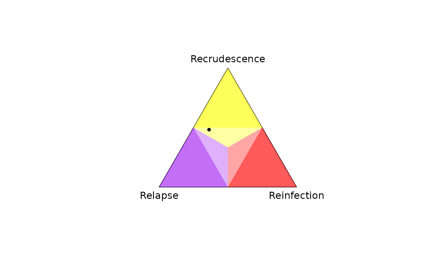
# Arbitrarily named alleles, plotting per-recurrence posteriors
y <- list(enrolment = list(marker1 = c("Tinky Winky", "Dipsy"),
                          marker2 = c("Tinky Winky", "Laa-Laa", "Po")),
          recurrence = list(marker1 = "Tinky Winky",
                          marker2 = "Laa-Laa"))
fs <- list(marker1 = c("Tinky Winky" = 0.4, "Dipsy" = 0.6),
           marker2 = c("Tinky Winky" = 0.1, "Laa-Laa" = 0.1, "Po" = 0.8))
plot_simplex(p.coords = compute_posterior(y, fs, progress.bar = FALSE)$marg)
#> Number of valid relationship graphs (RGs) is 30
#> Computing log p(Y|RG) for 30 RGs
#> Finding log-likelihood of each vector of recurrence states
#> 



# Episode names are cosmetic: "r1_prior" is returned for "r2"
y <- list(enrol = list(m1 = NA), r2 = list(m1 = NA), r1 = list(m1 = NA))
prior <- matrix(c(0.6,0.7,0.2,0.3,0.2,0), ncol = 3,
                dimnames = list(c("r1_prior", "r2_prior"), c("C", "L", "I")))
suppressMessages(compute_posterior(y, fs = list(m1 = c(a = 1)), prior))$marg
#> Warning: Data and prior episode names disagree
#> Warning: Marker m1 has data on fewer than two episodes
#> Warning: Episodes enrol & r2 & r1 have no data
#>      C   L   I
#> r2 0.6 0.2 0.2
#> r1 0.7 0.3 0.0
prior
#>            C   L   I
#> r1_prior 0.6 0.2 0.2
#> r2_prior 0.7 0.3 0.0


# Prior is returned when all data are missing
y_missing <- list(enrol = list(m1 = NA), recur = list(m1 = NA))
suppressMessages(compute_posterior(y_missing, fs = list(m1 = c("A" = 1))))
#> Warning: Marker m1 has data on fewer than two episodes
#> Warning: Episodes enrol & recur have no data
#> $marg
#>               C         L         I
#> recur 0.3333333 0.3333333 0.3333333
#> 
#> $joint
#>         C         L         I 
#> 0.3333333 0.3333333 0.3333333 
#> 


# Return of the prior re-weighted to the exclusion of recrudescence:
suppressMessages(compute_posterior(y_missing, fs = list(m1 = c("A" = 1)),
                 MOIs = c(1,2)))
#> Warning: Marker m1 has data on fewer than two episodes
#> Warning: Episodes enrol & recur have no data
#> $marg
#>       C   L   I
#> recur 0 0.5 0.5
#> 
#> $joint
#>   C   L   I 
#> 0.0 0.5 0.5 
#> 
# (Recrudescing parasites are clones of previous blood-stage parasites. The
# Pv3R model assumes no within-host de-novo mutations and perfect allele
# detection. As such, recrudescence is incompatible with an MOI increase on
# the preceding infection.)


# Beware provision of unpaired data: the prior is not necessarily returned;
# for more details, see link above to "Understand posterior estimates"
y <- list(list(m1 = c('1', '2')), list(m1 = NA))
fs <- list(m1 = c('1' = 0.5, '2' = 0.5))
suppressMessages(compute_posterior(y, fs))$marg
#> Warning: Marker m1 has data on fewer than two episodes
#> Warning: 
#>              C         L         I
#> [1,] 0.3292683 0.3414634 0.3292683